Introduction
Machine learning algorithms are only as effective as their data (both training data and predictor variables). Unfortunately, remote sensing analysts and researchers often train machine learning models with data that force the algorithm to make biased predictions. In addition, remote sensing analysts and researchers use the variable (feature) importance to show valuable predictor variables that contribute the most to the model. However, variable importance metrics are often biased when the predictor variables are highly correlated. This high collinearity often leads to selecting suboptimal predictor variables in the model. Therefore, remote sensing analysts and researchers cannot tell the valuable predictor variables and those that are not. This blog post will briefly discuss how Shapley values can be applied in modeling forest above-ground biomass (AGB) to understand critical predictor variables and minimize bias.
What are Shapley Values?

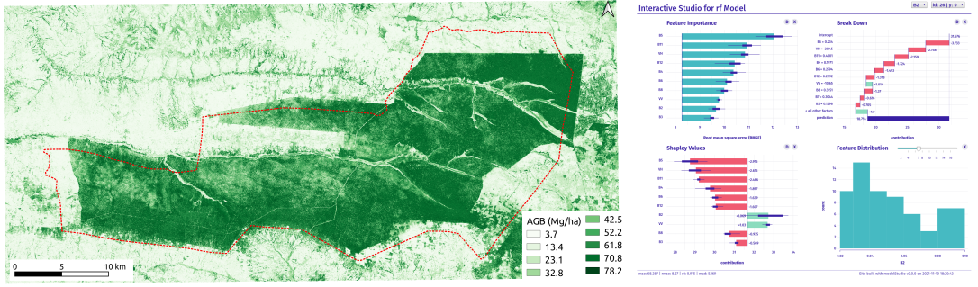
The Shapley values estimate the importance of an individual player in a collaborative team. In other words, Shapley values provide a solution to assigning a fair or reasonable reward to each player. In modeling forest AGB, remote sensing researchers can apply Shapley values to allocate feature importance fairly in a given model. The Shapley values can show how the predictor variables contribute to the model’s prediction with different magnitude and signs. The figure below shows Shapley values representing estimates of variable importance (extent of the contribution) and prediction direction (sign). For example, predictor variables with positive signs contribute to the prediction of forest AGB, whereas those with negative signs decrease the model’s prediction.
Insights into Model Performance and Errors
Shapley values can help us better understand the contribution of the predictor variables and gain insights into the model errors. In the above figure, the variable importance identified band 5 (from the rainy season Sentinel-2 data), elevation (Muf_DEM1), and forest height (b1) as the most important predictor variables. However, the Shapley analysis revealed that the same predictor variables negatively impacted the prediction. In contrast, slope, two Sentinel-1 bands (VV.1 and VV.2), and normalized difference vegetation index (nd) contributed positively to the prediction of forest AGB. The Shapley analysis illustrates the limitations of using only the variable importance and the complexity of the random forest model. Therefore, remote sensing analysts and researchers need to use explainable machine learning tools to gain insights into the contribution of the predictor variables and model errors.
Data and Procedure
This blog tutorial will use a random forest model to estimate forest AGB. We will use an improved forest AGB training data set, Sentinel-1 and Sentinel-2 data, normalized difference vegetation index, the Global Land Analysis and Discovery (GLAD) tree height, ALOS-derived elevation, and slope data. We will use Mafungautsi Forest Reserve in Zimbabwe as a test site in this post. Readers can access the blog tutorial and data in the links below.
Readers can also click the links below to check the AGB map interactive dashboard.
Next Steps
I have prepared an introductory guide to perform explainable machine learning.

If you want to learn more about explainable machine learning, please download the guide for free at: